1. Design of Metamaterials using Topology Optimization
Property-based topology optimization designs a microstructure whose homogenized stiffness matches a target tensor. Use it to synthesize metamaterial unit cells with SIMP, filters and sensitivity weighting, then to verify the result with a full-scale finite-element model.
- Reading time
- 9 min
- Length
- 1,577 words
- Updated
- Sep 15, 2026
- Total views
- --
1. Topology Optimization using the target mechanical property
There are two main reference for the property-based topology optimization, including [1] and [2]
We already know the homogenization issue and the energy-based homogenization from [3] and [4]. So we start from the Section4 of [1:1], which is the optimization model.
(1) Optimization Model
We use the SIMP approach for the design of metamaterials, the density is defined as :
The Formulation of optimization should be :
Here,
(2) FE Analysis Process
Firstly, to check how periodic boundary conditions are applied and solved, for example MATLAB code of it, see [5] for details.
For the FE analysis, we can use follows :
We note
Reduction to the
The prescribed displacement and periodic relation leave
Therefore, the complete displacement vector is :
Premultiplication by
Using the symmetry of
After solving this system, recover the slave-boundary displacement and the reaction by
Matrix Reduction
For a general matrix with some known variables, we can use following steps to reduce it to a lower-rank problem :we don't want
to appear in the final form.
- If the
is partially known, express the as : where
is unknown vectors
- Then we need another matrix
the new form is reached.
This transformation is also directly applicable in symbolic software such as SymPy, Mathematica, or the MATLAB Symbolic Math Toolbox. In an FE solver, the same relation is generally imposed with a multi-point constraint (MPC).
%%%%%%%%%%%%%%%%%% FE-ANALYSIS  %%%%%%%%%%%%%%
sK = reshape(KE(:)*(Emin+xPhys(:)'.^penal*(E0-Emin)),64*nelx*nely,1);
K = sparse(iK,jK,sK); K = (K+K')/2;
Kr = [K(d2,d2), K(d2,d3)+K(d2,d4); K(d3,d2)+K(d4,d2), K(d3,d3)+K(d4,d3)+K(d3,d4)+K(d4,d4)];
U(d1,:) = ufixed;
U([d2,d3],:) = Kr\(-[K(d2,d1); K(d3,d1)+K(d4,d1)]*ufixed-[K(d2,d4); K(d3,d4)+K(d4,d4)]*wfixed);
U(d4,:) = U(d3,:)+wfixed;(3) Derivatives of Homogenized Stiffness matrix
We compute the derivation against every element density
From [2:1], we know that we have (1.1.1)[3:1], then :
Then we have
To compute above expression in dolfinx, it's an anisotropic computation, the stress of it should be computed by mat.mu and mat.lmbda to compute the stress :
(4) Application cases for the design of meta-materials
For example, we want to maximize the bulk modulus[6] in (1.7)[6:1], we will minimize the negative of it :
Or the shear modulus in (2.4)[6:2], it is :
the
We also note besides (1.4.1~2), the article[2:2] gives a more general form, reads :
where
If we want to reach a material with negative-poission's ratio, we want to minimize the Poisson's ratio
The above expression is not the general Poisson ratio of a homogenized 2D cell. It recovers the original 3D isotropic Poisson ratio only when (C) is an isotropic plane-strain stiffness tensor.
Since the optimized microstructure is generally anisotropic, so that conversion no longer applies.
The definition under uniaxial loading in direction 1 is :
We let the homogenized compliance as :
Then the general expression of Poisson's ratio are :
and :
To get the poisson's ratio, we can use :
C_sym = 0.5 * (C_H + C_H.T)
S_H = np.linalg.inv(C_sym)In the original essay, the target function is set as:
where
xnew = max(0,max(x-move,min(1, min(x+move,x.*(-dc./dv/lmid)))));Why setting this target function reasonable ? Under uniaxial stress in direction 1, we have :
To maximize
while minimize and , the target is reasonable.
2. Implementation by FEniCSx
(1) Indexing rule of Sphinx
- In the dolfinx, every component has a
ufl_shapeattribute, so they have multiple components, We can access the components directly by indexing. For example, 2d strain/stressis (2x2) matrix and 3d strain is (3x3) matrix.
u_sol[0]   # x displacement
u_sol[1]   # y displacement

# they returns a Indexed object
# For example, to compute the magnitude in another space, we can use interpolate + expression :
V_mag = fem.functionspace(msh, ("CG", 1))
u_magnitude = fem.Function(V_mag, name="displacement_magnitude")
u_magnitude.interpolate(
    fem.Expression(
        ufl.sqrt(u_sol[0] ** 2 + u_sol[1] ** 2),  # also ufl.inner(u_sol, u_sol)
        V_mag.element.interpolation_points,
    )
)
u_magnitude.x.scatter_forward()
plot_function_pv(u_magnitude, title="displacement magnitude")(2) Stress Computation for anisotropic materials
So, having the C66 matrix
In implementation, we firstly, need two transfer functions to transfer the tensor notation to voigt notation, as given in [8], then, we can implement the stress computation as :
def stress_e_c66 (C66, eps):
	eps_voigt = tensor_to_voigt(eps, engineering_shear=True)
	C_const = ufl.as_matrix(C)
	sigma_voigt = ufl.dot(
        C_ufl,
	    eps_voigt,
    )
return voigt_to_tensor(sigma_voigt, dim)(3) Computation of Derivatives of Stiffness Matrix
We know from (1.3.3) that, we can compute the derivatives by :
For sensitivity of stiffness matrix, we have following computations :
def effective_stiffness_sensitivity(
    homo: CellHomogenization,
    rho: np.ndarray,
) -> tuple[np.ndarray, np.ndarray]:
    r"""Assemble the elementwise derivatives of the homogenized stiffness.

    .. math::
        \frac{\partial C^H_{IJ}}{\partial \rho_e}
        = \frac{1}{\lvert Y \rvert} \int_{Y_e} \eta^{(I)} : \mathbb{C}_{,\rho} : \eta^{(J)} \, dY.

    where :math:`I = ij,  J = kl`

    The EBHM correctors use
    :math:`\eta^{(I)} = E^{(I)} - \varepsilon(\chi^{(I)})`.
    """
    homo.update_density(rho)
    mat, msh = homo.mat, homo.msh
    V0 = fem.functionspace(msh, ("DG", 0))
    C_H, correctors = homo.solve_ebhm(return_u_solu=True)
    dim = homo.dim
    comps = len(unit_strain_tensors(dim=dim))
    if len(correctors) != comps:
        raise ValueError("Number of correctors must match the Voigt components.")

    unit_strains = unit_strain_tensors(dim=dim)
    eta = [
        fem.Constant(msh, unit_strains[I]) - strain(correctors[I])
        for I in range(comps)
    ]
    unit_vec = ufl.TestFunction(V0)
    dC_H_drho = np.zeros((comps, comps, len(rho)))

    dscale = (
        homo.penalty
        * (homo.rho_max - homo.rho_min)
        * rho ** (homo.penalty - 1.0)
    )
    for I, eta_I in enumerate(eta):
        for J, eta_J in enumerate(eta):
            Q = ufl.inner(stress_e(mat.mu, mat.lmbda, eta_I), eta_J)
            Q_vec = fem.assemble_vector(
                fem.form(Q * unit_vec * ufl.dx)
            )
            dC_H_drho[I, J, :] = dscale * Q_vec.array / homo.vol
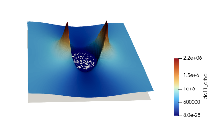
return C_H, dC_H_drhoWe note here we use the bulk modulus in (1.4.1) as the objective, After getting the derivative, we can plot and check the components, the [0, 0] component of the gradient
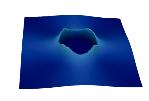
while the [0, 1] component is like :
(4) Essential problems
1) Filter Configurations
Firstly we have, for (2.3.1) :
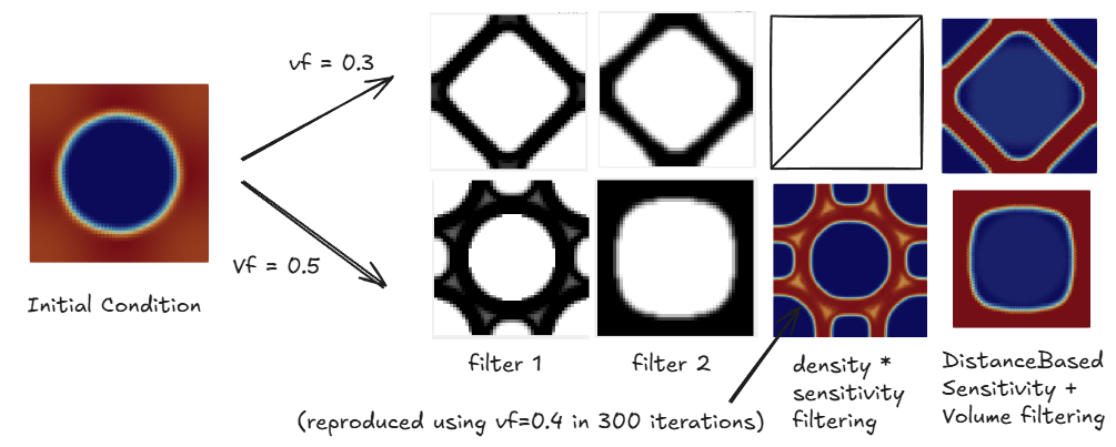
For the density filtering, we only use the density filtering only to get the final physical density, if we apply the filter in the middle process, the filter may hinder the density transformation process, or even deteriorate the results.
If we use the physical (filtered) density to compute the
We have following result :
In the code example, we can implement this filtering process by following :
density_filter = DistanceBasedFilter(
    msh,
    rmin=filter_radius * min_mesh_size(msh),
    p=1.0,
    filter_type="element",
)
C_H, dC_H_drho = effective_stiffness_sensitivity(
	homo,
	rho_physical,
)
# C^H_1111 + C^H_1122 + C^H_2211 + C^H_2222
bulk_stiffness = float(np.sum(C_H[:2, :2]))  # float(C_H[0, 1])
dJ_drho = -np.sum(dC_H_drho[:2, :2, :], axis=(0, 1))  # - dC_H_drho[0, 1, :]
dJ_drho_filtered = density_filter.apply_adjoint(dJ_drho)
vols_filtered = density_filter.apply_adjoint(vols)
Lmbda = optimization_criteria(
	rho=rho_design,
	dc_drho=dJ_drho_filtered,
	elem_vols=vols_filtered,
	vol_frac=volume_fraction,
	zeta=move_limit,
	precision=1e-6,
	lmbda_range=(1e-30, 1e30),
	rho_min=rho_min,
	rho_max=rho_max,
)In the essay that we references, the article provides 2 types of filters. In our
cellgenpackage, theDistanceBasedFilterapplying at both sensitivity and volume is same tofilter2. According to the article, there are 2 types of filters, given in the following code :matlab%% FILTERING/MODIFICATION OF SENSITIVITIES if ft == 1 dc(:) = H*(x(:).*dc(:))./Hs./max(1e-3,x(:)); elseif ft == 2 dc(:) = H*(dc(:)./Hs); dv(:) = H*(dv(:)./Hs); end
2) The crucial Initial Condition Problem
In the debugging process, one of the critical problem is the initial condition. This can simply be fixed by modifying the line as :
if sqrt((i-nelx/2-0.5)^2+(j-nely/2-0.5)^2) < min(nelx,nely)/3
%%%%%%%%%%%% set to follows %%%%%%%%%%%%
if sqrt((i-nelx/2-0.5)^2+(j-nely/2-0.5)^2) < 0.15 * nelx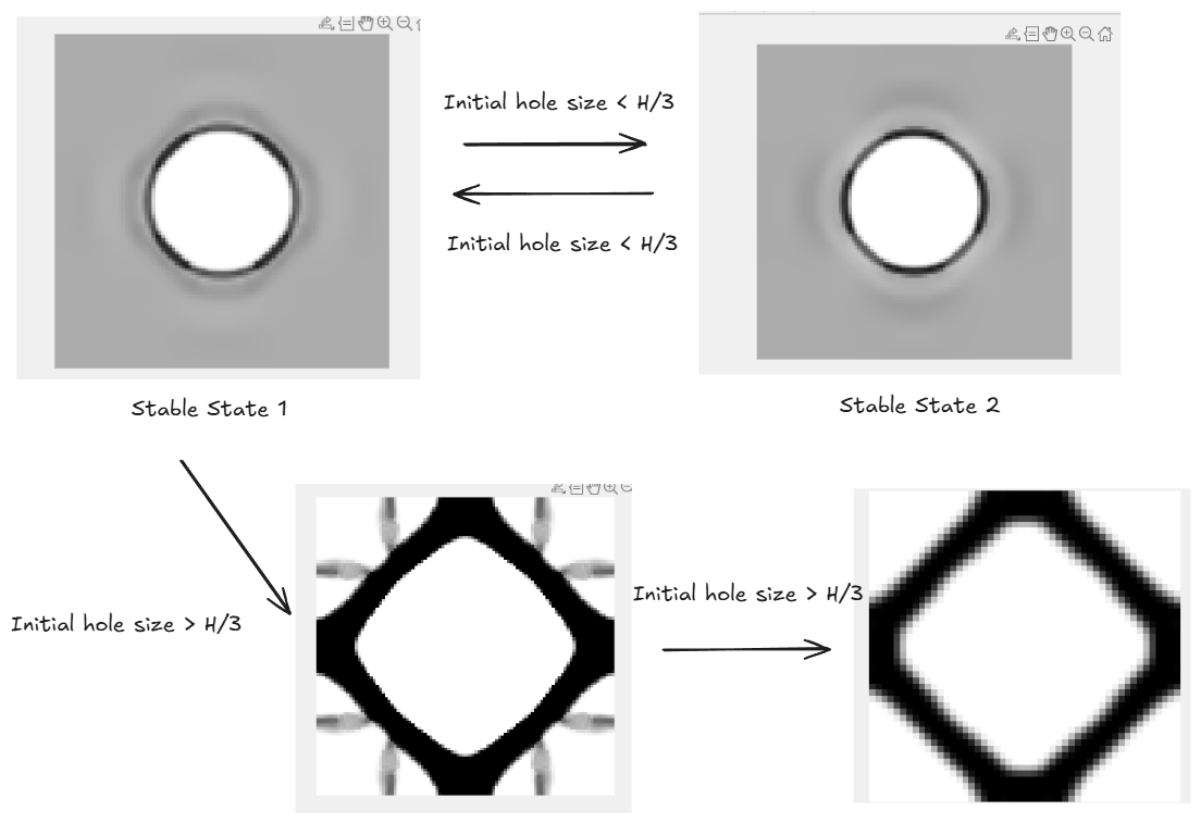
3) MMA problem for inner density increase
The unconservative MMA updates, while topX.m uses density-filtered OC bisection. MMA continued making large moves after the objective peaked, transferring density into the center. So, the OC optimizer is generally stabler than MMA optimizer.
We note that lower penalty is also beneficial. penalty = 3.5 -> 4 is a better choice than the penalty = 5.
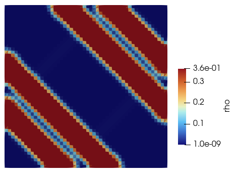
One of the problem is, the filter radius is also crucial. A good choice is 2, the result can be asymmetric. The following structure is reached by setting r=1.5 .
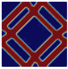
The following gives a result on
(5) Poisson's ratio
By the optimization of Poisson's ratio, we can still reach some materials with negative Poisson's ratio.
The generation configs is center hole radius 1/6, with following configs :
volume_fraction = 0.3
rho_min = 1e-9

config = UnitCellOptimProblemConfig(
	vol_frac=volume_fraction,
	max_iterations=150,
	result_dir=str(Path(__file__).parent),
	result_filename="microcell_top_design_density.xdmf",
	density_filename="microcell_top_design_best_density.npy",
	penalty=3.5,
	filter_radius=1.2,
	rho_min=rho_min,
	rho_max=1.0,
	move_limit=0.1,
	backend="mma",  # Use "oc" to select the optimality-criteria update.
	mma_auxiliary_penalty=1e5,
	mma_max_subproblem_iter=200,
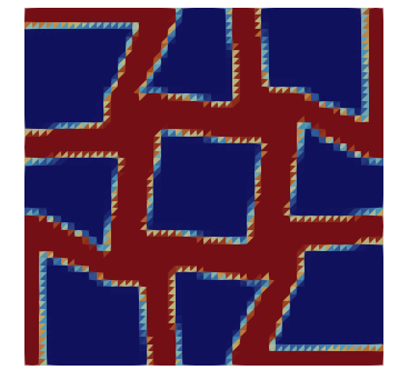
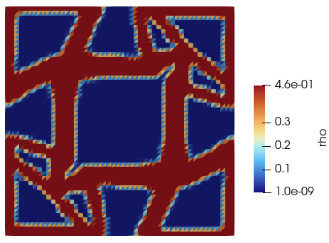
)Under these configurations, the poission's ratio is -0.5, resulting microstructure is given in Fig. 2.7 :
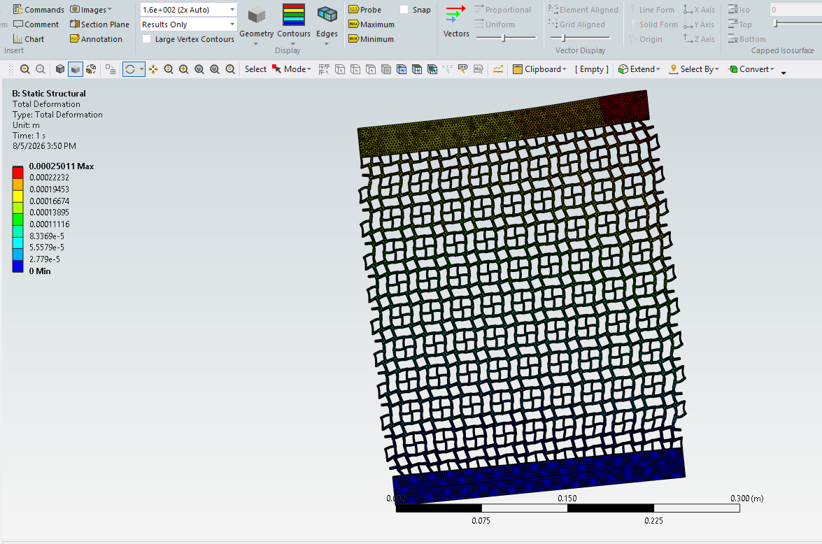
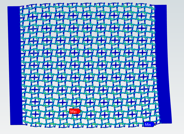
We can validate the auxetic properties by ANSYS using a lattice constructed by this cell :
Another typical configuration is:
def center_hole(x):
    return (x[0, :] - 0.5) ** 2 + (x[1, :] - 0.5) ** 2 < ((0.2) ** 2)

volume_fraction = 0.4
rho_min = 1e-9

config = UnitCellOptimProblemConfig(
	vol_frac=volume_fraction,
	max_iterations=150,
	result_dir=str(Path(__file__).parent),
	result_filename="microcell_top_design_density.xdmf",
	density_filename="microcell_top_design_best_density.npy",
	penalty=3.5,
	filter_p=0.7,
	filter_radius=1.0,
	rho_min=rho_min,
	rho_max=1.0,
	move_limit=0.1,
	backend="mma",  # Use "oc" to select the optimality-criteria update.
	mma_auxiliary_penalty=1e5,
	mma_max_subproblem_iter=200,
)The optimization result under 50x50 resolutions are given in Fig. 2.9
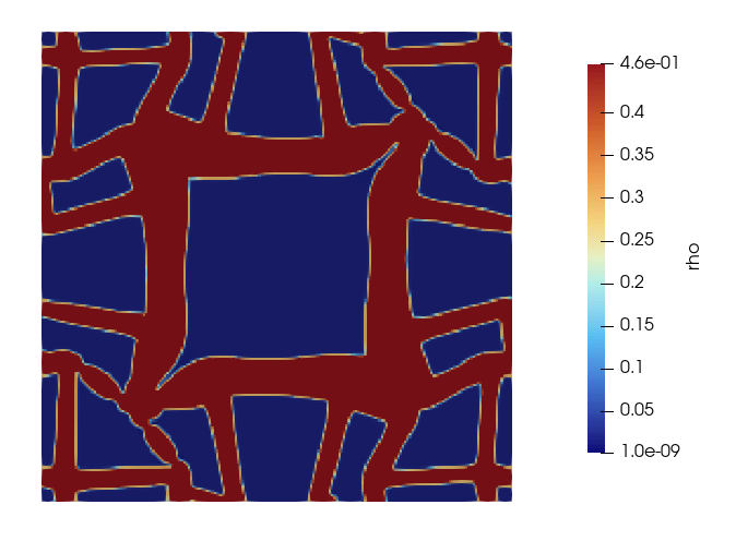
We note fhat we may need to increase the resolution into 200x200 for a detailed structure, We can get the structure with more detailed structure layout, given by following picture :
Xia, Liang, and Piotr Breitkopf. “Design of Materials Using Topology Optimization and Energy-Based Homogenization Approach in Matlab.” Structural and Multidisciplinary Optimization 52, no. 6 (2015): 1229–41. https://doi.org/10.1007/s00158-015-1294-0. ↩︎ ↩︎
Gao, Jie, Hao Li, Zhen Luo, Liang Gao, and Al Et. “Topology Optimization of Micro-Structured Materials Featured with the Specific Mechanical Properties.” International Journal of Computational Methods, ahead of print, 2019. https://doi.org/10.1142/S021987621850144X. ↩︎ ↩︎ ↩︎
EBHM ↩︎
PBC ↩︎